Instructor: Dean Gabriel
Let's consider two genetic loci, A & B, and two alleles each (A & a; B & b): What are the possible combinations of these four? Even though they can combine from parental gametes in 16 possible ways, there are only 9 genetic combinations. At equilibrium in a population, they would be present in the same proportions as would be expected from writing out the calculated products of their independent equilibrium frequencies. For example, if we had determined for the 'A' locus that p = 2/3 and q =1/3 and also independently for the 'B' locus that p = 3/4 and q = 1/4, then we could calculate the actual frequency of AABB as (2/3)2 X (3/4)2 = 1/4, AABb as (2/3)2 X 2(3/4 X 1/4) = 2.67/16, AAbb as (2/3)2 X (1/4)2 = 4.44/16 etc.
At Equilibrium
AABB .25
AABb .17
AAbb .03
AaBB .25
AaBb .17
Aabb .03
aaBB .06
aaBb .04
aabb .01
1.0
But it can take a long time to arrive at these equilibrium frequencies. One can see from the hand out (Stern's Fig. 118) that if one starts with 100% AaBb in generation 1, then one reaches equilibrium at both loci in a single generation. However, this is an unusual case (in natural populations, but not in plant breeding, as we will soon see).. If we start out 50% AABB and 50% aabb, then in generation 1, 1/4 progeny will result from matings among AABB individuals, 1/2 from matings between AABB and aabb individuals, and 1/4 of the progeny from matings among aabb individuals. In other words, the homozygotes, by chance, are not contributing to any of the other 7 combinations, and there are a significant number of them. We see that it takes time to reach equilibrium with two alleles at each of two loci. There is a tendency of parental types to remain together that is unrelated to crossing over between genes, but rather is related to the fact that there are so many of the "parental" population types that they have a certain probability of mating among themselves, rather than with the other "parental" group population. In a population, this is called linkage disequilibrium.
What if the loci are linked? Then it takes even longer to reach equilibrium, because the loci are not independently assorting. There is a tendency of parental gene types to remain together for this added reason: crossing over. The physical linkage adds to the linkage disequilibrium of the population..
We have examined how alleles behave and are distributed in a population, and we've now looked in some detail at how gene frequencies achieve an equilibrium in populations and how these frequencies are affected by mating systems (random vs. assortative). We mentioned earlier some other effects on populations that now deserve mention. For example, how does a very rare allele, a mutation with no selective advantage or disadvantage, become established in a population? Fisher calculated the probability of survival of a mutation appearing in a single human individual, and without any selective advantage or disadvantage. His calculations depend upon the number of offspring the individual has, but basically, the probability of survival (refer Table 117) of a mutant allele arising in an individual declines rapidly over time. Why? It's mainly because human beings produce limited numbers of offspring, and there are very good chances that a given human will not mate, will be sterile, and even if he/she does produce offspring, there is a 50% chance that a mutation will not be passed along. Note the 47% probability that the mutation will go extinct in one generation. Even if it does not go extinct in one generation, the limited number of offspring that bear the mutation also have a high chance of not passing the mutation along, for all the reasons true for the previous generation.
However, if a mutant allele gets passed along to more than one descendant, the likelihood of survival becomes much greater (refer table 118). Of course, there are many thousands of loci, and within each locus, many thousands of possible mutations. What happens to most of them? They may never be passed along, and this has a very high probability with each early generation. Most mutations, then, become extinct, but a few can and do survive. This type of calculation was examined with great interest by mutationists, who you will remember favored the idea that chance alone provided the variation observed in nature. However, the likelihood of any one particular mutation accumulating by chance as rapidly as observed by Luria & Delbrook for a favorable mutation was extreme, and it was population genetic arguments that proved that some other force, selection, had to be involved.
In fact, theoretical calculations demonstrated that for dominant mutations with selective value (either positive or negative), selection had a very immediate effect, and for recessive mutations, selection had a delayed, but very strong effect also, taking any particular mutation with positive selective value from basically 0 to nearly 100%. Selection operates very slowly on recessive mutations when they are rare, but once they become appreciable in number, they rapidly increase to nearly 100%
Once an allele is established, can its frequency change? As we have seen, the answer is clearly YES, it can, and this phenomenon is called genetic drift,
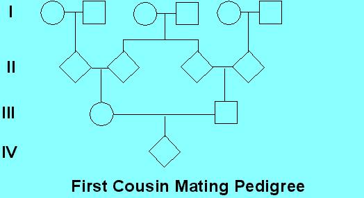
Consider as given that the female III-1 is heterozygous Aa, let's say for albinism. What is the likelihood that her mate, the male III-2, is also Aa? Obviously, for III-1 to be Aa, she had to get 'a' from one of her parents. This means there is a 1/2 chance of 'a' being inherited from parent II-2. IF II-2 is Aa, then one of his parents (I-3 or I-4) had to have the allele, and if one of them had the allele, they could have passed it to II-3 with a probability of 1/2. IF II-3 is also Aa, then it could be passed to III-2 with a probability of 1/2. For II-2 AND II-3 AND III-2 to all have Aa, the probability is 1/2 X 1/2 X 1/2 = 1/8. Now compare that fixed 1/8 probability if III-1 mates with someone other than her cousin. We previously calculated 2pq, the frequency of heterozygotes for one of the albinism loci, to be 1/100. If she mates with her cousin, since she is Aa for sure, and the chances that he is also Aa are 1/8, the chance that they will have an albino child (aa) are 1/8 X 1/4 = 1/32. If she mates with an unrelated male, however, the chance that they will have an albino child are 1/100 X 1/4 = 1/400. It is important to realize that this 1/32 chance of homozygosity is true for each and every gene! If you have 10,000 genes, then on average 312.5 recessive genes that are common to your particular family are going to be made homozygous if you mate with your first cousin. That is, not only are 312.5 recessive genes going to be homozygous, but 312.5 genes are going to be identical. Rare defects (and mutations) that occur in a family can be revealed in really personally devastating ways. As we have seen, such defects rarely cause trouble and rarely become established in a population.
Consider the following data from Japan, France and the U.S. on mental
defects:
| Population | From unrelated marriages | From 1st cousin marriages |
| France | 3.5% | 12.8% |
| Japan | 8.5% | 11.7% |
| U.S. | 9.8% | 16.15% |
Note that regardless of reporting levels overall, there is a much higher rate of defects resulting from 1st cousin marriages.
In Utah, between the years 1847 and 1870, the percentage of cousin marriages
rose from 1/2 to nearly 100%. By 1930, the marriages to cousins had
dropped to nearly 0. This is likely due to a break down of isolation,
increase of urbanization and the discovery and application of Mendel's
laws to populations.
One way to measure the extent of inbreeding is by using the coefficient
of inbreeding F, which is a measure of probability that inbreeding has
occurred and to what extent. 0 = no inbreeding and 1 = complete inbreeding.
Inbreeding coefficients are of great consequence to animal breeders, because
many "elite" breeding lines of cattle, horses and dogs are highly inbred,
and the coefficient of inbreeding is calculated for particular individual
animals. They are also valuable to genetics counselors, at both an
individual and population level. For individuals, the inbreeding
coefficient F is the probability of having inherited a given allele
from a common ancestor and F = (1/2)n, where n is the number
of ancestors from an individual through one parent and back again
through the other (shortest path). For example, in the above example
involving first cousins, the path to calculate the F value for the individual
"IV-1" goes through III-1 to II-2, II-3 and III-4, giving n = 4 and F =
1/16. (Note this is a different question from the question
asked before of the probability that IV-1 would be homozygous at a given
locus if you knew that one of the first cousin parents was heterozygous
at the locus). For brother-sister unions, the F value of offspring
is 1/4. For uncle-niece & aunt-nephew unions, F = 1/8.
For second cousins, F = 1/64. These values assume that the ancestors
in common are not themselves inbred. If they are, the formula becomes,
F = (1/2)n (1 +FA), where FA refers to
the ancestral inbreeding coefficient. If there is more than one common
ancestor, the total inbreeding coefficient is the sum of the F values calculated
for each ancestor.
The average inbreeding level in a population may be calculated and provides useful comparisons. Say 1,000 people had 909 individuals of random parentage, 1 from uncle-neice matings, 30 from 1st cousin matings and 60 from 2nd cousin matings.
The average F = (909 X 0) + (1 X 1/8) + (30 X 1/16) + (60 X 1/64)
= 0.00294.
1,000
These population values have been calculated for a number of populations,
including:
| Population | Period | Number Marriages | F value |
| Rio de Janeiro (urban) | 1946-1956 | 1,172 | 0.00044 |
| Bombay (urban) | 1950 | 512 | 0.0092 |
| Andrha Pradesh (rural) | 1957-1958 | 6,945 | 0.032 |
Note that in the above data, the lowest values (least inbreeding) are
obtained in urban areas. Why?